Antimicrobial Resistance in Biofilms Formed During Secondary Food Processing of Meat and Meat Products
Antimicrobial Resistance in Biofilms: Findings
This sections discusses the findings of the research project.
3.1 Sampling Strategy
3.1.1 Literature review
Full details of the literature review are provided in Appendix 1. Studies were reviewed to understand the prevalence of AMR bacteria in different meats. However, it is hard to draw firm conclusions because the studies reviewed were often not designed to investigate the differences among meat types, and indeed only two studies testing multiple meat types presented the results with sufficient clarity. From the 74 studies examined in the previous literature review [10] and assessed here, it appears, albeit from limited data and without a formal statistical assessment, that poultry may have a higher prevalence of AMR bacteria than beef or pork. Only one study was found that assessed mutton, and this was at slaughter [39].
In terms of the locations to sample within factories, few relevant papers were identified. However, Wagner et al [40] was extremely informative, providing a comprehensive list of sites sampled, and identifying those sites in which biofilms were and were not detected. Identified biofilm hotspots were slicers, conveyors, drains, hoses and a wagon. These are all locations which were likely to be available for sampling in the factories selected for the current study.
The laboratory studies were also informative. All bacteria tested were able to form biofilms on all tested materials, meaning no surface materials could be ruled out of sampling. Meat juices were frequently found to enhance biofilm growth, so meat contact surfaces (or surfaces on to which meat-based liquids can drip) were deemed profitable sites to sample. It was suggested (though not explicitly tested by any of the studies) that surfaces with microscopic scratches or abrasions may be adherence points for biofilm formation (similar to the “fabric valleys” on conveyor belts) [41]. Older or more well used equipment may therefore be more likely to house biofilms.
3.2 Sampling Methodology Development
3.2.1 Swabbing methods
Undiluted DNA extracts from all samples taken with dry swabs produced an amplicon, whereas undiluted extracts from samples taken with wet swabs did not produce amplicons. However, diluting the DNA from the wet swabs did allow successful PCR, perhaps indicating the presence of PCR inhibitors. The extracts were also quantified by Qubit measurement. The mean DNA concentration in the extracts was lower for dry swabs than for wet swabs, at 0.25ng/µl and 1.52 ng/µl respectively (mean across the different extraction methods).
The fact that reliable amplification took place from dry swab samples, and that this method meant there was a lower chance of sample mix up or contamination (as swabs can be used straight from the packet, rather than needing to be pre-moistened), led to the decision to use dry swabs for sampling. For extraction, the PCR results indicated no real difference in amplicon generation between the four different extraction methods, so going forward, the simplest method of massaging the swabs in 1 x PBS prior to centrifugation was chosen.
The 16S amplicon results of the storage experiment indicated that swabs could be stored at 4°C for 6 hours (to simulate time between swabbing at the factory and return to the lab), then storage at -40°C for 8 days with no deterioration of the DNA.
The comparison of the use of Biofinder, no use of Biofinder, and use of Biofinder followed by rinsing prior to sampling generated the following result (Table 3).
Table 3. The number of sequence reads and nucleotide bases obtained from biofinder, non-biofinder and rinsed biofinder samples (one of each), and the sequences attributed to E. coli and Pseudomonas.
| Sample | Non-Biofinder | Biofinder | Biofinder-rinse |
|---|---|---|---|
| Raw Reads | 91720 | 147355 | 199099 |
| Bases | 261581479 | 334340419 | 360427845 |
| Median Length | 2560 | 1990 | 1580 |
| E. coli Raw Reads | 78981 | 129906 | 168581 |
| E. coli Bases | 207381308 | 277339007 | 290864906 |
| E. coli Bases (%) | 79.28 | 82.95 | 80.70 |
| Pseudomonas Raw Reads | 4609 | 552 | 4594 |
| Pseudomonas Bases | 7581053 | 896952 | 7181586 |
| Pseudomonas Bases (%) | 2.90 | 0.27 | 1.99 |
Following these experiments, it was concluded that the use of Biofinder and subsequent rinsing with water reduced the amount of DNA that could be extracted, but still generated sufficient DNA for sequencing, and both taxa present in the sample could be identified at similar levels to the sample not treated with Biofinder.
3.2.2 Sampling SOP
The sampling SOP developed is presented in Appendix 2. The critical step to ensure biofilms are sampled is the pre-rinsing of the surface with molecular grade water prior to sampling. An attempt was made to ensure a uniform sampling effort by prescribing the area and method of swabbing. After feedback received from factories that Biofinder was foaming at a minority of sampling locations, factories were permitted to sample from non-foaming locations, so long as the rinsing protocol was followed.
3.3 Sampling
3.3.1 Biofilm samples
One hundred and forty-six biofilm samples were received from the four factories and processed for metagenome sequencing (Appendix 3). These are summarised in Table 4.
Table 4 Numbers of metagenome-sequenced biofilm samples from each factory.
| Factory ID used in this report | Number of samples |
|---|---|
| Factory A | 46 |
| Factory B | 24 |
| Factory C | 30 |
| Factory D | 46 |
3.4 Sequencing Results
3.4.1 Illumina
3.4.1.1 Quality control and assembly
A total of ~14.6 billion raw paired-end reads were generated. After quality control steps and the removal of non-bacterial reads ~8.4 billion remained. All samples generated enough data to produce assemblies, save for samples 095 and 117, which produced ~35 thousand and 37 raw reads respectively.
The remaining samples had between 0% to 99% of reads removed as non-bacterial, with a median of 19%. After assembly, all but the above two samples had an assembly size of at least 8Mb, but with a wide distribution of lengths. The N50 statistic for each sample ranged from 222 bp to 12,430 bp.
The sequencing, decontamination and assembly statistics are provided in Appendix 4.
3.4.2 Nanopore
3.4.2.1 Quality Control and Assembly
A total of ~8.5 million reads (just under 101 gigabases) were generated, with an average PHRED quality score of 13.2 (4.8% error rate) and an average median read length 865.2 nucleotides observed (control samples excluded from averages). Assemblies were generated for all samples, but a large number of contigs were removed due to contamination with large amounts of metazoan sequence for 6 samples (077, 089, 107, 116, 131, 222). These samples were subsequently removed from further analysis, leaving 15 assemblies with n50 values ranging from 7,484 to 56,433.
3.4.3 Hybrid Assembly
All 15 samples selected for hybrid assembly were successful, producing a large number of contigs, with n50 values ranging from 561 to 14,253.
Note: The 15 samples which were used for a comparison between Illumina, Nanopore and hybrid assembly methods will henceforth be referred to as the benchmarking subset.
3.4.4 ARG Detection
For each sample, the RGI software lists matches between a reference ARG sequence and a contig sequence. Note that one contig can appear in more than one match, since long contigs may match multiple ARGs. Conversely, the same ARG sequence can be present on more than one unique contig sequence.
Each unique ARG type is identified by a unique ID in the ARO ontology [26].
RGI identifies ARGs using one of several 'models', depending on the nature of the ARG. The majority involve sequence similarity of the implied protein sequences ('protein homolog model'). Some ARGs have a resistance function due to particular point mutations distinguishing them from non-resistance genes with near-identical sequences. These are treated with a 'protein variant model' which takes account of this. There is also an 'rRNA gene variant model', since the same consideration applies to some rRNA, i.e. non-coding genes. Other ARGs are considered to only have a resistance function in the context of their overexpression ('protein overexpression model').
Here, we present analyses of the RGI output collectively. Results of interest include the distribution of numbers of unique ARGs in the set of samples, and conversely the number of samples in which each unique ARG has been detected.
In 132 of the 144 samples, the mean percentage identity of the unfiltered ARG matches was ≥ 97% (≥ 98% in 116, and ≥ 99% in 77 samples). However, the mean coverage breadth of the reference sequences was much lower (Appendix 5). The following results all refer to the matches passing our filter (minimum 80% coverage breadth and identity), except where otherwise stated.
3.4.4.1 Filtered RGI results
The following refers to the identity and coverage breadth-filtered data, for example, which is restricted to ARG matches which have at least 80% sequence identity and account for at least 80% of the length of the reference ARG sequence.
Overall, the filtered RGI results showed that the sequences of 144 unique ARGs (unique ARO IDs) were detected in the full set of experimental samples; none occurred in the controls (Figure 1). The highest number of ARGs in any one sample (sample 084) was 71. This sample was taken from a stainless steel surface in factory D, that was mainly exposed to chicken burgers, mince and a small amount of pork burgers. Ten samples had over 20 unique ARGs detected. Fifty of the biofilm samples had no ARGs detected.
For each sample, the numbers of unique ARG names, and total number of ARG matches (each ARG may occur more than once), are listed in Appendix 6.
The full list of 144 ARGs and their drug classes, resistance mechanisms and AMR gene families (as designated in the ARO ontology) are in Appendix 7. Many ARGs are assigned to multiple drug classes, mechanisms or families in ARO. Table 6 lists the incidence of drug classes among the 144 ARGs.
Figure 1. The distribution of the number of unique ARGs (ARO IDs) occurring in each sample (filtered RGI data). (a) Colours indicate processing plant. (b) Colours indicate meat type.
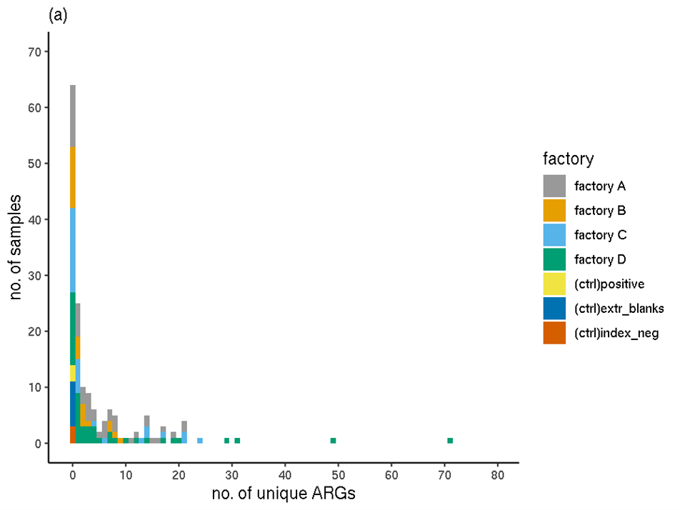

The distributions of the number of unique ARGs in each sample were compared between factories using a Wilcoxon Rank Sum Test (Table 5) with a Bonferroni-Holm adjustment for multiple comparisons. No significant (p<0.05) difference was detected between any pairs of factories. The distribution of ARGs in factories A and B appeared most different but this observation was not significant (p=0.073).
Table 5: Quantiles of the number of ARGs per sample and the significance of differences in distributions between factories
| Factory | Number of ARGs per sample - Median | Number of ARGs per sample - 80% Quantile | Significance of difference B | Significance of difference C | Significance of D |
|---|---|---|---|---|---|
| A | 3 | 11.2 | 0.073 | 0.33 | 1.00 |
| B | 1 | 2.4 | NA | 1.00 | 0.33 |
| C | 0.5 | 13.2 | NA | NA | 0.37 |
| D | 2 | 10.4 | NA | NA | NA |
Table 6. ARO drug classes of the 144 unique ARGs which are positive in any sample(s) after the 80%-identity, 80%-coverage filter of the RGI output.
| ARO drug class | no. of unique ARGs |
|---|---|
| aminoglycoside antibiotic | 16 |
| carbapenem; cephalosporin; penam | 15 |
| diaminopyrimidine antibiotic | 10 |
| tetracycline antibiotic | 10 |
| fluoroquinolone antibiotic | 8 |
| macrolide antibiotic; lincosamide antibiotic; streptogramin antibiotic | 7 |
| carbapenem | 6 |
| peptide antibiotic | 6 |
| phenicol antibiotic | 6 |
| fosfomycin | 5 |
| glycopeptide antibiotic | 5 |
| disinfecting agents and intercalating dyes | 3 |
| fluoroquinolone antibiotic; monobactam; carbapenem; cephalosporin; glycylcycline; cephamycin; penam; tetracycline antibiotic; rifamycin antibiotic; phenicol antibiotic; triclosan; penem | 3 |
| rifamycin antibiotic | 3 |
| cephalosporin; penam | 2 |
| fluoroquinolone antibiotic; cephalosporin; glycylcycline; penam; tetracycline antibiotic; rifamycin antibiotic; phenicol antibiotic; triclosan | 2 |
| fluoroquinolone antibiotic; tetracycline antibiotic | 2 |
| lincosamide antibiotic | 2 |
| macrolide antibiotic | 2 |
| macrolide antibiotic; aminoglycoside antibiotic; cephalosporin; tetracycline antibiotic; peptide antibiotic; rifamycin antibiotic | 2 |
| macrolide antibiotic; fluoroquinolone antibiotic; monobactam; carbapenem; cephalosporin; cephamycin; penam; tetracycline antibiotic; peptide antibiotic; aminocoumarin antibiotic; diaminopyrimidine antibiotic; sulfonamide antibiotic; phenicol antibiotic; penem | 2 |
| macrolide antibiotic; lincosamide antibiotic | 2 |
| macrolide antibiotic; lincosamide antibiotic; streptogramin antibiotic; tetracycline antibiotic; oxazolidinone antibiotic; phenicol antibiotic; pleuromutilin antibiotic | 2 |
| nucleoside antibiotic | 2 |
| penam | 2 |
| sulfonamide antibiotic | 2 |
| acridine dye; disinfecting agents and intercalating dyes | 1 |
| aminoglycoside antibiotic; aminocoumarin antibiotic | 1 |
| cephalosporin | 1 |
| elfamycin antibiotic | 1 |
| fluoroquinolone antibiotic; cephalosporin; penam; tetracycline antibiotic; peptide antibiotic; acridine dye; disinfecting agents and intercalating dyes | 1 |
| fluoroquinolone antibiotic; diaminopyrimidine antibiotic; phenicol antibiotic | 1 |
| fusidic acid | 1 |
| macrolide antibiotic; fluoroquinolone antibiotic; aminoglycoside antibiotic; carbapenem; cephalosporin; penam; peptide antibiotic; penem | 1 |
| macrolide antibiotic; fluoroquinolone antibiotic; lincosamide antibiotic; carbapenem; cephalosporin; tetracycline antibiotic; rifamycin antibiotic; diaminopyrimidine antibiotic; phenicol antibiotic; penem | 1 |
| macrolide antibiotic; fluoroquinolone antibiotic; penam | 1 |
| macrolide antibiotic; fluoroquinolone antibiotic; tetracycline antibiotic; phenicol antibiotic | 1 |
| macrolide antibiotic; penam | 1 |
| monobactam; carbapenem; cephalosporin; penam | 1 |
| monobactam; carbapenem; penam | 1 |
| monobactam; cephalosporin; penam | 1 |
| monobactam; cephalosporin; penam; penem | 1 |
| nitroimidazole antibiotic | 1 |
3.4.4.2 Number of samples in which each unique ARG sequence was detected (filtered RGI results)
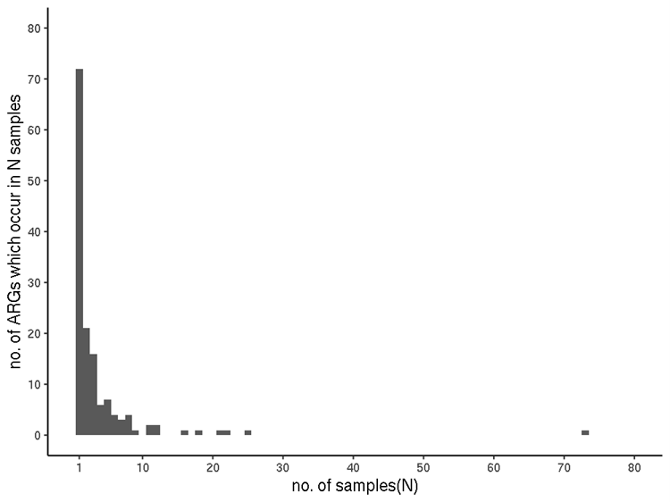
Most ARGs were only seen once. The sequences of almost half of all identified ARGs (71 of the 144) were detected in only a single sample each, coincidentally the same number as the maximum number of ARGs identified in any one sample. Twenty-one occur in two samples, 16 in three, six ARGs occur in four samples. Nineteen ARGs occur in 5 to 9 samples, with 10 occurring in 11 or more (Figure 2). The outlier in 73 samples is rsmA (ARO:3005069) (drug classes: "fluoroquinolone antibiotic; diaminopyrimidine antibiotic; phenicol antibiotic").
Figure 2. Sample-incidence of each ARG (filtered RGI data).
3.4.4.3 ARG incidence (filtered RGI results)
In metagenomic assemblies, the incidence of an ARG in one sample refers to the variety of contexts (assembled contigs/scaffolds) in which it occurs, and not to abundance. For simplicity, the previous summaries of ARG sequences detected in samples was in terms of unique ARGs (defined by unique ARO terms). However, each unique ARG can occur one or more times in each sample; i.e., there can be one or more contig sequences in which the ARG can be detected (indeed, it is possible for a unique ARG sequence to be detected in more than one location within a long contig, in principle). Highly similar, or even identical instances of the same ARG may occur within a sample's set of assembled contigs, for several reasons.
A biological explanation is that the same ARG may occur in the sample in different genomic contexts (i.e. in different positions in the same genome, or in different strains or species, where the flanking DNA may be different).
In theory, with perfect sequencing and assembly, if there were only a single biological context within one sample then all sequencing reads, which sample the ARG and flanking DNA, would be incorporated into a single contig. However, sequencing errors and imperfect assemblies can prevent this.
Therefore, multiple instances of detection of the same ARG sequence in one sample are not uncommon, due to both biological and technical reasons.
For any sample, the total incidence, in terms of positive contig-ARG matches, is therefore the sum of all of the individual ARG instances. The mean of this incidence sum for all samples for each production plant and for each meat type are shown in Table 7 and Table 8 respectively.
3.4.5 ARG quantification (filtered RGI results)
The sum of a sample's TPM values for all ARGs (ORFs matching ARGs; in this case, fulfilling the 80%-identity, 80%-coverage criteria) represents the total number of biological sequences estimated to be ARGs, out of every million sequences. This includes protein-coding genes, but not other genes (such ribosomal RNA gene variants which confer resistance).
Like the incidence values, the TPM values are indicative. The normalisation applied enables within-sample comparison of abundances, not between-sample, due to the proportional nature of the metric. Therefore, mean TPMs calculated across multiple samples must be treated with caution.
The means of these sample TPM sums are presented in Table 7 and Table 8 for each production plant and each meat type respectively.
Note that when this estimation is performed, all ORFs, of all contigs, are considered, irrespective of whether those ORFs correspond to ARGs, and irrespective of any filtering. Thus, a given ARG in a given sample has the same TPM value in both the unfiltered and filtered results - assuming it passes the filter. However, the total TPM value can be different in filtered versus unfiltered - because in the filtered data, TPMs for ARGs no longer included (due to insufficient sequence identity and/or ARG coverage breadth) will not contribute to the sum.
Table 7. Mean per-sample incidence and mean per-sample estimated quantities, for each production plant.
| Factory | Mean incidence of each sample | Mean TPM of each sample |
|---|---|---|
| Factory A | 5.6 | 36.86 |
| Factory B | 1.9 | 40.77 |
| Factory C | 4.7 | 21.19 |
| Factory D | 7.4 | 18.00 |
Table 8. Mean per-sample incidence and mean per-sample estimated quantities, for each meat type.
| Meat type | Mean incidence of each sample | Mean TPB of each sample |
|---|---|---|
| Chicken | 3.5 | 16.93 |
| Pork | 1.6 | 6.11 |
| Chicken and pork | 8.6 | 21.73 |
| None | 7.0 | 63.12 |
The all-sample mean TPM values for the 22 ARGs with the highest means (≥0.1) are shown in Table 9.
Table 9. Mean TPM values across all samples, for each unique ARG (filtered RGI results). For brevity, an arbitrary cut-off of TPM = 0.1 has been used, with only those ARGs above the threshold shown.
| ARO | Samples | TPM |
|---|---|---|
| 3005069 | rsmA | 18.78208 |
| 3000816 | mtrA | 1.17788 |
| 3003784 | Mycobacterium tuberculosis intrinsic murA conferring resistance to fosfomycin | 0.76577 |
| 3005009 | qacE | 0.67982 |
| 3004682 | aadA27 | 0.550938 |
| 3003836 | qacH | 0.542619 |
| 3002639 | APH(3'')-Ib | 0.542598 |
| 3005098 | qacL | 0.486602 |
| 3005036 | BLMT | 0.447909 |
| 3002884 | iri | 0.334873 |
| 3002660 | APH(6)-Id | 0.313656 |
| 3002950 | vanXB | 0.29559 |
| 3000025 | patB | 0.243801 |
| 3000518 | CRP | 0.194949 |
| 3003369 | Escherichia coli EF-Tu mutants conferring resistance to Pulvomycin | 0.189135 |
| 3000178 | tet(K) | 0.160697 |
| 3002823 | ErmH | 0.151185 |
| 3002554 | AAC(6')-Ig | 0.150475 |
| 3000175 | tet(H) | 0.136387 |
| 3001714 | OXA-215 | 0.122966 |
| 3004597 | Klebsiella pneumoniae KpnH | 0.112272 |
| 3000781 | adeJ | 0.106347 |
3.4.6 Co-location
ARG co-location was defined as more than one ARG identified on the same contig. Using this metric, a total of 52 (22 for the benchmarking subset), 0 and 24 co-locating ARGs were identified from the Illumina, Nanopore and hybrid assemblies respectively. Full ARG co-location tables for Illumina, Nanopore, and hybrid assemblies are supplied in Appendix 8.
3.4.7 Mobile Genetic Elements (MGEs)
A total of 1,209 contigs from the long-reads assemblies and 11,150 contigs from the short-reads assemblies contained hits to at least 1 MGE. Each sample had at least 1 MGE identified in it. MGE blast results are supplied in Appendix 9.
3.4.8 Metagenomically Assembled Genomes (MAGs)
Of the 15 hybrid assemblies, 3 assemblies contained contigs that were of length 1.5Mb or greater - samples 047, 053 and 087. The single contig from sample 047 was identified as Parvibaculum lavamentivorans.
3.4.9 Taxonomic Identification
Across all samples, a total of 243 genera were identified by Metaphlan3. The most frequently occurring genera were Parvibaculum, Cutibacterium and Methylobacterium, identified in 148, 124 and 119 samples respectively, which were all genera also present in the control samples. When genera which were identified in control samples were removed, 227 genera remained, with the most frequently occurring genera being Rhodococcus, Kocuria and Pseudomonas, identified in 82, 82 and 78 samples respectively. A matrix detailed the identified genera and their relative abundances are supplied in Appendix 9.
3.4.10 Hybrid Assembly Comparison
The benchmarking subset of assemblies were compared, with a focus on the quality of the assemblies. Assembly quality can be roughly estimated through metrics such as the number of contigs (fewer is better), total size of the assembly (larger is often better), contig L50 (smaller is better), contig N50 (larger is better) and the maximum contig size. L50 is defined as the count of the number of contigs whose length makes up half of the assembly/genome. N50 is defined as the sequence length of the shortest contig at half the length of the genome/assembly. The maximum contig size can give an indication of whether an entire genome has been captured in a single contig.
Of note, is the fact that the Nanopore assemblies are often generated from substantially less data than the Illumina assemblies. As such, the assembly size for Nanopore assemblies will be smaller than the hybrid or Illumina assemblies. For this same reason, the number of contigs is also likely be smaller. Additionally, the Nanopore assembler used, Flye, specifies a minimum length requirement, therefore a number of shorter reads will be excluded from the initial assembly steps.
When Illumina and hybrid assemblies alone are compared for number of contigs, L50 and N50, 15/15 hybrid assemblies have fewer contigs, 14/15 have a better L50 and 13/15 have a better N50, suggesting that the addition of longer reads leads to a more contiguous assembly.
3.5 qPCR Results
3.5.1 Quantification of selected AMR genes using qPCR
The qPCR cycle threshold (CT) values for the calibration standards were plotted against the log of the copy number to generate a standard curve. In the samples where target amplification was detected, the CT value was used to derive a measure of the copy numbers by extrapolation from the standard curve.
Quantitative real-time PCR assays exhibit a Limit of Quantification (LOQ) below which CT values are not sufficiently reproducible to reliably estimate the copy number. While we have not formally assessed the LOQ for each of the assays, values calculated at less than 100 copies/µl should be regarded as falling below the LOQ and not reliable estimates of copy number in this study.
These estimates for the copy number values are presented in Appendix 11.
Following the sequencing experiments there was sufficient sample extract remaining in 118 samples to conduct the qPCR analysis. For the 16S gene we obtained valid qPCR results for 117 of the samples, with the calculated copy numbers ranging from 103 to more than 106 copies/µl. For the AMR tet(B) gene we detected only low quantities (less than 100 copies/µl) and in only eleven of the samples. These values for tet(B) should be considered below the LOQ and therefore regarded as qualitative results. With the sul(I) gene, we detected its presence in all the 118 samples tested. In the majority of samples, the values of sul(I) were below the LOQ, but a significant minority of samples showed values above this threshold. To investigate this further we compared the sul(I) copy numbers to those obtained for 16S in the same samples. This is illustrated in Figure 3 below.
Figure 3. Comparison of copy number estimates for the 16S and sul(I) genes. Scatter plot of copy number estimates for each sample with generally increasing trend to higher sul(I) values with increasing 16S copies detected. The marked circle encompasses points where the sul(I) is raised above this general trend.
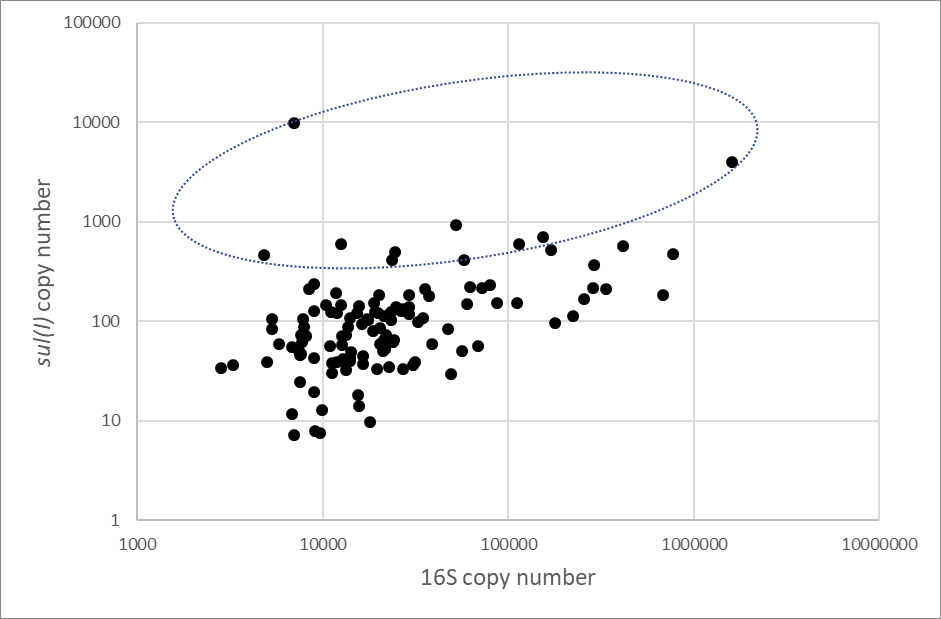
The sul(I) assay used in this study may be amplifying a low level of ‘non-specific’ product which is detected by the SYBRTM Green dye in all biofilm sample extracts (albeit these ‘non-specific’ amplicons produce the expected Tm in the 84.05±0.25C range similarly to genuine sul(I) amplicons). This would suggest that in the majority of samples the sul(I) detections are not genuine and are more reflective of the quantity of bacteria in the biofilm sample. There are, however, a number of sample where the sul(I) detections are raised above this background level and which are more likely to have resulted from genuine detections. We would estimate that there are 8-10 samples where the sul(I) detection is more likely to be genuine.
3.5.2 Normalisation and comparison to metagenomic data
As stated in section 3.4.5, TPM values represent proportions of each gene or DNA fragment among all of those sequenced. Ultimately this is because the DNA sequence data is compositional and does not provide information on absolute quantities.
We therefore attempted to use the qPCR results for the two specific ARGs tet(B) and sul(I), and the general bacterial qPCR (16S rRNA gene), as external references to calibrate the TPM values for each of the samples for which qPCR data was available. We also incorporated the ORF sequences which in silico PCR (ecoPCR software) had indicated to be tet(B) or sul(I). These would not necessarily all have been found by the RGI/CARD analysis, especially after we had applied the strict filter to these results. We confirmed that sequences corresponding exactly to the primer pairs used for tet(B) and sul(I) are present in the CARD database. Each pair is present in one reference sequence, which have the expected gene annotations.
Additionally, as 16S data was available for all of the samples assayed by qPCR, and we had calculated TPM values for all of the in silico PCR 16S sequences, we used these data to calibrate the total-ARG TPM values for these 117 samples. The numbers of samples positive by each method is shown in Table 10.
Table 10 Numbers of samples positive for each gene by sequence analysis and qPCR. 16S refers to the sequences amplified by the 515-806 primers used in this study and not to specific variants which are in the CARD database.
| Sample |
unfiltered RGI |
filtered RGI | ecoPCR | qPCR | qPCR, est ≥ 500 copies/μl |
|---|---|---|---|---|---|
| tet(B) | 19 | 0 | 1 | 11 | 0 |
| sul(I) | 40 | 7 | 11 | 117 | 9 |
| 16S | N/A | N/A | 144 | 117 | 117 |
3.5.2.1 tet(B)
Prior to filtering, the tet(B) RGI results showed a small number of samples being positive; however, all of them had very poor coverage of the reference sequence and did not pass the filter. The single ecoPCR in silico amplicon sequence was checked against the NCBI nt database, but no similarity to a known sequence was found. This indicates that this sequence is probably in a misassembled region of a metagenomic contig, flanked by matching primer sequences. The metagenomes are therefore negative for genuine tet(B) sequences, which is largely consistent with the qPCR results. We therefore did not consider tet(B) further.
3.5.2.2 sul(I) in relation to 16S
Similar numbers of samples were positive for sul(I) in the filtered RGI and ecoPCR results (Table 10). The 7 filtered RGI-positive are a subset of the 11 ecoPCR-positive. We confirmed that the other 4 were all RGI-positive before filtering. Each of the 11 had one in silico amplicon and we examined these to confirm that they are highly similar to the expected sequence. qPCR analysis had been applied to three of these 11 samples. The positive samples and their metagenome-estimated sul(I) relative abundances (TPM values) and copy numbers estimated from qPCR are shown in Table 11. This also shows the TPM values calculated for all of the ecoPCR 16S sequences, and the qPCR-estimated 16S copy numbers for those samples which were assayed.
Table 11. In silico positive ORFs and abundances, and qPCR abundances of sul(I) and 16S for the 11 samples positive for a predicted sul(I) amplicon. Cells marked with a dash indicate samples which were not assayed with qPCR.
| sample ID | sul(I): filtered RGI ORFs | sul(I): ecoPCR ORFs | sul(I): rel. abund. (TPM) | sul(I): est. copy no. | 16S: rel. abund. (TPM) | 16S: rel. abund. (TPM) sul(I): copy no/TPM | sul(I): copy no/TPM | 16S: copy no/TPM |
|---|---|---|---|---|---|---|---|---|
| 053 | 1 | 1 | 0.05 | - | 317.80 | - | - | - |
| 078 | 0 | 1 | 0.05 | - | 455.43 | - | - | - |
| 079 | 1 | 1 | 0.51 | - | 600.71 | - | - | - |
| 080 | 0 | 1 | 0.15 | 4,034 | 604.50 | 1,607.670 | 26.944.9 | 2,659.5 |
| 083 | 1 | 1 | 6.12 | - | 660.79 | - | - | - |
| 084 | 1 | 1 | 0.63 | - | 667.76 | - | - | - |
| 085 | 1 | 1 | 1.68 | - | 567.77 | - | - | - |
| 088 | 1 | 1 | 0.18 | - | 520.67 | - | - | - |
| 101 | 1 | 1 | 0.29 | 601 | 298.37 | 113,579 | 2,038.4 | 380.7 |
| 137 | 0 | 1 | 0.26 | - | 258.21 | - | - | - |
| 223 | 0 | 1 | 0.32 | 412 | 104.53 | 23,647 | 1,275.2 | 226.2 |
In principle for any gene, the ratio of the copy number (absolute, per μl) to the TPM (relative abundance) represents a scale factor to convert the TPM values to copy number equivalents. This is expected to vary considerably between samples, because the absolute amounts of DNA in the original samples may differ considerably. This ratio is shown in Table 11 for the three samples with qPCR data. If all of the sequencing data, TPM estimates and qPCR copy numbers are consistent, then this scale factor should be the same for all genes. However, the same ratios for 16S differ from the sul(I) in all three samples, by a factor of 5 to 10.
This indicates that if the qPCR data is indicative of the true abundances, the metagenomic sequencing and/or abundance calculations are not sampling these two genes proportionally. Although two of the samples' sul(I) copy numbers are close to the limit considered to give reliable estimates (one is below it), the third (sample 080) has the second highest sul(I) copy number in any sample. This sample had a high number of metagenome sequencing reads (123 million following contaminant removal).
3.5.2.3 Total ARGs in relation to 16S
We used the same approach as in the previous section, to estimate copy number equivalents for all protein-coding ARGs collectively. This could be done for all samples to which qPCR had been applied for the 16S gene, and thus had a copy number:TPM ratio available for 16S. The same principle was applied as for the sul(I) gene, but here the sum of all ARG TPMs was used for each sample, rather than the TPM of a single gene. This was obtained by summing the KALLISTO-output TPMs for all ORFs which featured a positive RGI prediction which passed our identity/coverage filter. Multiplying this sum by the 16S copy number:TPM ratio thus applies a sample-specific scaling. In theory, the result is a copy-number equivalent measure for the set of any/all ARGs, collectively, which can be compared between samples. This relies on the assumption that the ratio would be generally similar for these ARG genes as for 16S, which was found not to hold for sul(I), albeit with very few data points available (previous section). The results of this normalisation should therefore be treated as indicative only. For the 118 samples involved, the results are shown in Appendix 11.
In summary:
scale factor = 16S copy no. / TPM (1)
normalised total ARG abundance = scale factor x total ARG TPM (2)
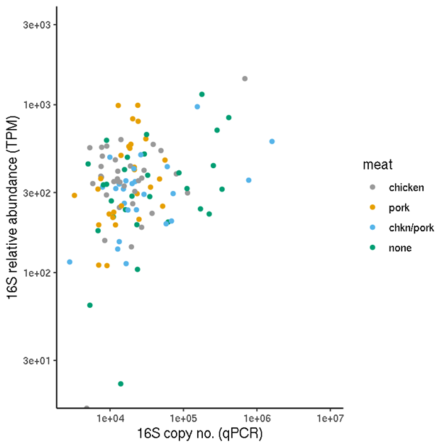
Figure 4 shows that the relationship (1) between 16S copy number from qPCR, and the 16S TPM values appear not to be random. There are no samples with high copy number estimates and low TPM. Nonetheless, as expected there is considerable variation in the ratio (used for the normalisation), particularly to TPM values greater than around 200.
Figure 4. Abundances of 16S gene in samples which were assayed by qPCR. Copy numbers (copy no/ μl) were obtained from qPCR. Relative abundances were calculated from metagenomic sequencing.
The unnormalised relative abundance values (TPM) should in principle not be compared between samples if absolute comparisons are of interest. One comparison of interest is therefore the normalised (2) values versus the unnormalised TPM (Figure 5). This shows that for this data set, there is a reasonable correlation between the two.
Figure 5. Comparison of estimated total-ARG copy numbers and total ARG relative abundances for each sample. The copy numbers were obtained by normalising the relative abundances by a sample-specific scale factor obtained from the 16S abundance analysis.
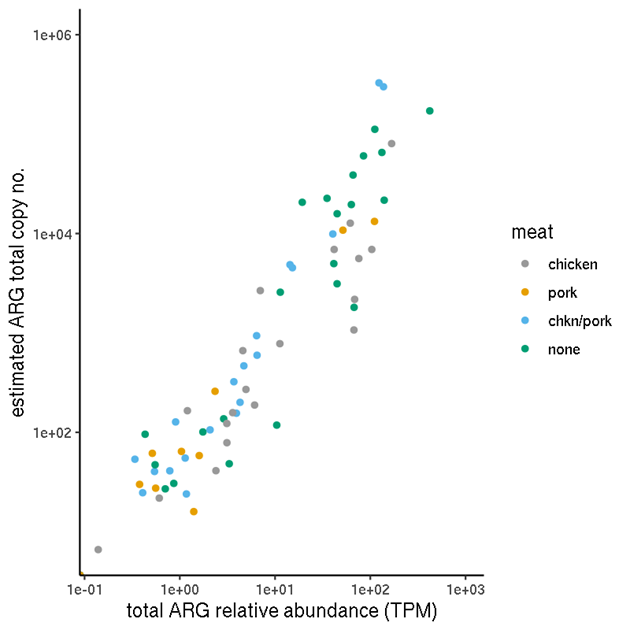
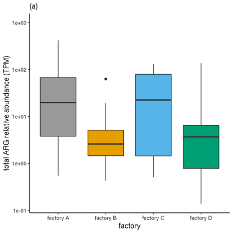
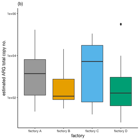
Figure 6 shows a comparison of the unnormalised TPM abundance values and the normalised abundances, for samples categorised by factory. Figure 7 Figure 7 shows the same for samples by meat type.
Figure 6. Total ARG abundances for each factory. (a) Unnormalised relative abundances. (b) Normalised abundances (estimated copy numbers per μl).
3.6 AMR burden from the UK diet and the possible link to biofilms
In this section, we consider the implications for UK dietary sources of ARGs. Existing information on AMR detected in retail meat samples is first summarised, for comparison.
Collection of the biofilms samples was designed to be representative of the UK diet as far as possible. However, there were some practical constraints, so we include a discussion of the total UK consumption of the relevant meat types and what this means for the representativeness of the sampled biofilms.
3.6.1 AMR phenotype of E. coli isolates data from EU harmonised surveys
The focus here is on the most recent UK data compiled by the FSA. Sampling was designed to represent 80% of the retail market share and 80% population coverage. In the most recent UK survey at least 300 samples were collected for each of 3 retail meat categories (beef, pork, poultry). Summary tables are presented below for fresh retail samples of UK Beef (Table 12), Pork (Table 13) and Chicken (Table 14) collected between 2015 and 2019. The type of samples collected varied between years. The proportion of positive samples is much higher for chicken than for other meat types.
Table 12. Summary of UK Beef samples 2015-2019 from the EU harmonised surveys
| Year (UK data) | Total beef samples | ESBL CTX | AmpC | ESBL CTX + AmpC |
|---|---|---|---|---|
| 2015 | 312 | 1 | 1 | 0 |
| 2017 | 314 | 1 | 1 | 0 |
| 2019 | 289 | 1 | 0 | 0 |
Table 13. Summary of UK Pork samples 2015-2019 from the EU harmonised surveys
| Year (UK data) | Total pork samples | ESBL CTX | AmpC | ESBL CTX + AmpC |
| 2015 | 312 | 1 | 1 | 0 |
| 2017 | 310 | 0 | 1 | 0 |
| 2019 | 285 | 2 | 1 | 0 |
Table 14. Summary of UK Chicken samples 2015-2019 from the EU harmonised surveys
| Year (UK data) | Total chicken samples | ESBL CTX | AmpC | ESBL CTX + AmpC |
|---|---|---|---|---|
| 2016 | 313 | 75 | 49 | 2 |
| 2018 | 309 | 23 | 16 | 3 |
Some additional information is provided by the reports linked in Section 2.8 that may be relevant. For example, in 2019 none of the isolates obtained from UK samples were carpabenamese-resistant or colistin-resistant (mcr-1, mcr-2, mcr-3 are the mobile colistin resistant genes tested for). Also, although 315 beef and 313 UK pork samples were collected in 2019, not all were suitable for reporting due to technical issues. In 2018, of the 309 chicken samples the type of chicken samples was listed, and these comprised 125 whole chicken, 112 chicken breasts and 72 other cuts, e.g. quarters, legs, thighs drumsticks. It was noted that the proportion of positive samples was higher for skin-off chicken, which may suggest the potential for cross contamination during the skin removal process. None of the isolates obtained from these samples were resistant to carbapenem or mcr-1, -2, or -3. Processed pre-prepared chicken including goujons, ready meals, marinated, breaded, battered, frozen or cooked chicken, were all excluded. The AMR samples collected in the current project, and the consumption survey data, do include these value-added poultry products, so there is a mismatch in the type of products when trying to link with the harmonised survey data. Additional contamination, or reductions in contamination, that may arise from these processes are therefore not represented in these data.
Table 15 lists those gene classes consistent with E. coli that were found in the biofilm samples, and/or those that were found in the survey of retail meat. There were 12 gene classes found in the biofilms samples but not recorded in the meat survey results.
Table 15. Gene classes found in biofilms samples, meat survey, or both, that are consistent with E. coli and were predicted to confer antibiotic resistance
| Found in meat survey but not biofilms | Found in biofilms samples but not meat survey | Found in biofilms samples and meat survey |
|---|---|---|
| polymyxin antibiotic | disinfecting agents and intercalating dyes, nitroimidazole antibiotic, elfamycin antibiotic, peptide antibiotic, penem, nucleoside antibiotic, monobactam, rifamycin antibiotic, triclosan, fosfomycin, glycopeptide antibiotic, acridine dye, aminocoumarin antibiotic |
aminoglycoside antibiotic, macrolide antibiotic, fluoroquinolone antibiotic, penam, carbapenem, cephalosporin, sulfonamide antibiotic, glycylcycline, cephamycin, tetracycline antibiotic, phenicol antibiotic, diaminopyrimidine antibiotic |
3.6.2 ARG detection in retail samples of chicken
In a scoping study of ARGs measured in retail chicken samples from the UK and Ireland [38] 76 samples were collected in total, including thigh (30), leg (27) and breast (19) meat portions. In Table 5 of McNeece et al (2014) the numbers of samples found to be positive for selected ARGs are listed. The ARGs found were: sul3 (6), tetD (12), tetE (18), cmlA1 (7), fox (44), catB8 (4) and cmy (62). The study used a statistical test to assess whether there was a difference in prevalence between each pair within the 3 source groups (UK-free range, IE-intensive, UK-intensive). Testing for bacteria was also reported in this paper, using Denaturing Gradient Gel Electrophoresis (DGGE) followed by sequencing of the products to identify some of the Gram-negative bacteria present. However, it was noted in the discussion that linking specific resistances to species is something that requires further work.
3.6.3 Consumption of Beef, Pork and Chicken products summarised from UK NDNS surveys
Trends in UK meat consumption (2008/9 – 2018/19) are addressed in Stewart et al. (2021) [42]. Within most population sub-groups, a reduction in overall meat consumption per day was inferred from the survey data. A statistically significant negative trend was reported for red meat, particularly for beef and sausages, but not in pork nor in burgers. For the current project, we attempted to reanalyse the UK consumption levels to extract information about specific relevant food types to answer questions about the UK burden from AMR in processed meat.
Table 16 shows the proportions of individuals within different subpopulations consuming the meat types of interest (beef, pork and poultry) after accounting for disaggregation into raw ingredients, summarised from the NDNS data. Minced beef, corned beef and cooked chicken slices are included as these make up significant proportions of the consumed items. Corned beef and wafer-thin chicken slices are types of ready-to-eat products, so the burden from these products is not considered here. Similarly, the consumption of pork will include a contribution from ready-to-eat ham. The burden from these and other ready-to-eat products was considered in a separate FSA project FS301050 [43].
Table 16. Proportion of individuals consuming one or more of the food types (Beef, Pork, Chicken)
| Population | Beef Total | Beef Mince | Beef Corned | Pork Total | Poultry* Total | Poultry* Wafer-thin chicken slices |
|---|---|---|---|---|---|---|
| Adults (18-64) | 62.8% | 41.3% | 4.2% | 78.9% | 88.2% | 6.2% |
| Older adults (65+) | 64.8% | 37.3% | 8.4% | 82% | 85.2% | 4.9% |
| Children (0-10) | 60.2% | 48.9% | 2.4% | 70.5% | 87.7% | 18.2% |
| Children (11-17) | 63.3% | 47.3% | 2.5% | 82.1% | 92.2% | 11.6% |
| All | 62.1% | 44.4% | 3.7% | 76.5% | 88.3% | 11.6% |
*The NDNS category is poultry and includes turkey consumptions
Plotting the amount of individual meat types as a function of the survey year also allowed us to investigate individual trends in products. Overall, we found that poultry is consumed by a larger proportion of the population than the other meat types, although pork is a close second. There is evidence of a general reduction in amounts of beef and pork consumed in recent years, but the average daily amounts of chicken consumption do not show a substantial change over the 11 years of the NDNS survey. The same conclusion was reported in Stewart et al (2021) where poultry and game birds were included as ‘white meat’ and found not to have changed significantly.
The individual meat types reported were also investigated, to help determine whether the collected biofilms samples were representative of current UK consumptions. We found that:
- Food names used to describe beef are: Steak, minced, topside, roast, cooked slices, ox tail, ox tongue, pastrami. Beef burgers did not appear in the summaries because these were classified using the raw ingredients (beef mince stewed) in the recipes database.
- Food names used to describe the types of pork consumed after recipe disaggregation are: Bacon (smoked, middle, back), Pork crackling, Pork shoulder, loin, belly, chops, tongue, ribs, Diced, Minced, Ham (smoked and unsmoked), Parma ham, Brawn, Polony, Haslet, Salami, Gammon, Roast pork roll/slices.
- The types of chicken described in the survey are: Chicken breast, roast, boiled, casserole, barbecued, slices, leg/drumsticks, wing, roll.
- The types of turkey consumed (although with far fewer consumers) are: Turkey breast, roast, slices, mince, roll/slices.
In summarising the proportion of individuals that are consumers within a (sub-) population, we have included wafer thin chicken slices as this is the only meat processing type that has a substantial number of consumers. We also note that this proportion is higher in children than in adults. As explained below, this does not necessarily represent chicken slices purchased as ready-to-eat chicken. Rather, it may be an artefact from using the recipes database because ‘wafer thin chicken slices’ appears there as a component of processed chicken products such as chicken burgers.
The summaries presented above relate to overall meat consumptions from broad classifications (beef, pork, poultry) and include ready to eat cooked foods and disaggregated ingredients from recipe dishes or from raw meat ingredients that cannot be linked to individual processed meat products directly. Even where a component food type might appear to represent a consumed product, they may also appear as part of a different product type. For example, there are recipes for chicken burger that include ‘chicken slices wafer thin not smoked’, so the chicken from the chicken burger is represented as wafer thin chicken slices. Other chicken burger recipes include ‘chicken cass light and dark meat only’ (sic). Coated chicken pieces takeaway is defined as ‘chicken boiled light meat only’. The translation from meat product to the raw primary meat types often leads to very different interpretations and makes it impossible to link the results directly to the processed meat samples. Another way to summarise the survey data that avoids these difficulties is to consider the product level descriptions without using the recipes. This was considered to be more useful for assessing the types of products purchased by consumers, and therefore the representativeness of the products sampled from the meat processing plants.
The NDNS was therefore re-examined to assess consumption by product type. The overall meat-related product categories in the NDNS are: Bacon and ham, Beef veal and dishes, Lamb and dishes, Pork and dishes, Chicken and turkey dishes, Coated chicken, Meat pies and pastries, Other meat and meat products, Sausages, Liver and dishes, Burgers and Kebabs. The numbers of consumers and some key individual products are shown in Table 17. These values give an indication of the relative numbers of individuals (from the total surveyed 18338) consuming particular food types. In principle, linking consumption of individual products to ARG levels in those products may provide information about the relative potential burden of AMR from biofilms linked to processing for those food types.
Table 17. Summaries of meat product consumptions recorded in the NDNS rolling program years 1-11 (2008/9-2018/19) combined with the DNSIYC for infants. The product groups are ordered by the total number of consumers. The total number of individuals in the data is 18338. Italicised food items are considered as ready to eat foods so are not in scope for the project. The bold food types are those processed in the sampled plants
| Meat product group | Number of consumers | Mean daily consumption (g) for consumers only | Main food types (by number of consumers) |
|---|---|---|---|
| Chicken and turkey dishes | 11863 | 92.9 | Chicken breast grilled (4051), Chicken roast (3830), Chicken boiled (2058), Wafer thin chicken slices (729) |
| Bacon and ham | 9831 | 42 | Ham, not smoked (6618) Bacon rashers grilled (3975) Bacon rashers fried (1151) |
| Beef veal and dishes | 8504 | 79.5 | Beef mince stewed (4039), Stewing steak stewed (954), Beef topside roast (938) |
| Sausages | 6753 | 57.9 | Pork sausages, grilled (4213), Frankfurter (593), Premium pork sausages (529), Chorizo (360) |
| Coated chicken | 4274 | 68.7 |
Chicken goujons (1178). Coated chicken pieces takeaway (1092),
|
| Meat pies and pastries | 3540 | 69.1 | Sausage roll (1456), Chicken pie frozen (345), Cornish pasty (199), Pork pie buffet (147) |
| Pork and dishes | 3149 | 62.6 | Pork loin chops grilled (939), Pork loin joint roasted (512), Diced pork stewed (279), Pork & beef meatballs (230) |
| Burgers and kebabs | 2372 | 62.4 | Beefburger 100% grilled (673), Beefburger economy grilled (441), Cheeseburger takeaway not ¼ pounder (402) |
| Other meat and meat products | 2276 | 43.1 | Salami (451), Corned beef not canned (363), Peperami (258), Corned beef (210), Black pudding fried (152) |
| Lamb and dishes | 2237 | 74.7 | Lamb leg roast (440), Lamb mince stewed (308), Lamb loin chops grilled (287), Lamb scrag and neck stewed (270) |
| Liver and dishes | 539 | 36.1 |
Liver pate plastic wrapped (225), |
3.6.4 Representativeness of the sampled factory areas for consumed food types
The meat processing factories include areas that process multiple product types, and so there is not a simple one-to-one relationship between biofilms and single food types. However, roughly classified meat types and numbers of samples associated with their processing can be listed as follows:
Factory A: added value chicken (4), brine (4), chicken + brine (3), chicken breast (11), diced chicken/fillets/portions (7), whole bird (3)
Factory B: pork (8), bacon (3), Wiltshire brine (2)
Factory C: pork (17), chicken (2), all meats: pork/chicken/beef (3)
Factory D: pork (5), chicken/chicken products (5), chicken and pork (25), chicken and pork sausages (6), chicken burgers/mince + pork burgers (2)
Food type descriptions included in the sample metadata and in the NDNS consumption diaries food are sometimes ambiguous and do not use a common coding system. There is some uncertainty therefore about the relative amounts of individual products processed. However, by comparing these terms against those products most commonly consumed in the survey (Table 17) it is possible to identify any missing food types. Beef mince products seem to be the most commonly consumed processed meat types that are not well represented in the processing types of our sampled factories. Other highly consumed meat products do seem to be represented, especially for the important category of chicken products, but also pork sausages and bacon. In some cases, there are highly consumed food product categories that are not described in sufficient detail to be able to determine whether they can be linked to one of our meat processing plant biofilm samples. The main examples seen in Table 17 are ‘chicken roast’ and ‘chicken boiled’.
3.6.5 Assessing population burden due to processing
If individual ARGs are identified and can be linked to one or more food types based on the classifications and summaries outlined above, then a simple process could be followed to estimate the proportion of individuals consuming those food types and therefore the proportion of individuals exposed to specific ARGs. This could be extended to consider the burden from broader general food types represented in the data (e.g. burden from chicken or burden from pork products). This general approach was used to estimate the measure of burden in the ready-to-eat food project FS301050. There are several limitations to this approach that mean it is a highly uncertain – and potentially misleading – estimate of the true overall burden. Within the current project it was therefore agreed that such an estimate would not be derived. Details of the uncertainties and suggestions for dealing with these are summarised in Section 4.2.7.
3.6.6 Comparing ARG prevalence in samples taken from chicken lines to ARG prevalence in bacteria detected in chicken
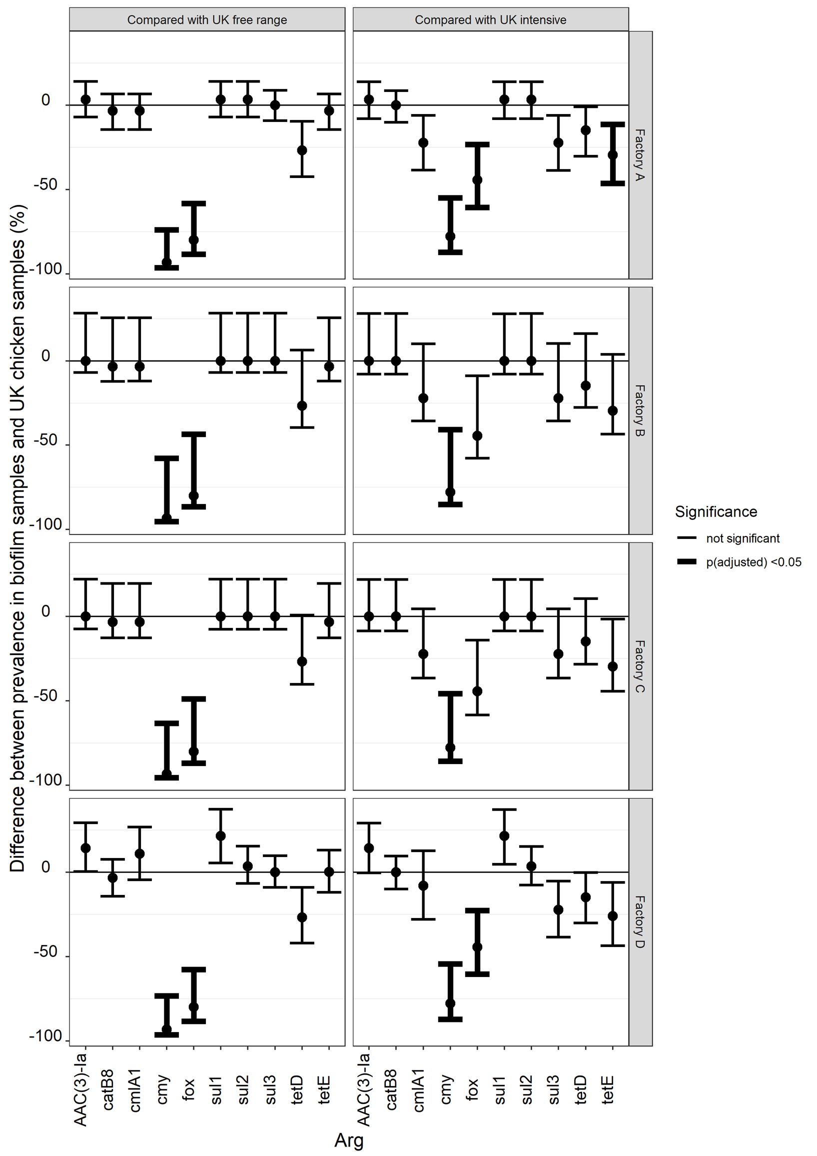
The proportion of national chicken samples which contained each of 47 ARGs [38] were compared with the proportion of biofilm samples in each factory that contained the same ARGs. Estimates of how much larger or smaller the factory biofilm proportion was compared with the national chicken proportion are shown in Figure 8 and Table 18. Of the 47 ARGs tested for on the array used for the chicken samples, five ARGs were detected in factory biofilms containing sequences consistent with Gram-negative bacteria: AAC(3)-Ia, cmlA1, sul1, sul2, tetE. Seven ARGs were detected in UK chicken samples catB8, cmlA1, cmy, fox, sul3, tetD, tetE. Although three ARGs were detected in factory samples that were not detected in chicken samples, the prevalence was low enough for the difference in proportions to be not significant (i.e. the underlying proportion in the population of chicken portions might be the same as the underlying proportion of biofilms). Cmy, fox and tetE were not detected in factories and were detected at prevalences that were significantly higher in UK chicken (again assuming that the prevalences are comparable). This analysis just shows that we didn't see that ARGs at high prevalences in biofilms were not present in similarly high proportions of chicken samples.
Figure 8: difference in prevalence of AMR in biofilm samples that contain Gram-negative bacteria and intensive UK chicken samples
Revision log
Published: 6 March 2023
Last updated: 8 March 2024